RHT

Rolling Hough Transform (RHT)

RHT is another image analysis method that is used to locate filamentary structures. In some respects it is a special case of the general template matching where the template is (in the simplest version) a linear line segment. Like in our template matching code, one starts the analysis by subtracting from the original image a filtered image (usually calculated using a top-hat filter). One is also comparing the resulting image to a “template”, a description of a linear structure. However, there are some fundamental differences:

(1) After subtraction of the filtered data, the image is thresholded at zero. Pixels with negative values are replaced with zeros and pixels with positive values are replaced with ones. In template matching this quantisation of the input data was not done.

(2) At each pixel position and a for number of position angles, one is effectively calculating the match between a “template” and the data. However, because the data now consists only of ones and zeros, the match (number of positive pixels matching a line) is not dependent on the original pixel intensities.

A description of RHT applied to astronomical image analysis can be found in Clark, Peek, & Putman (2014) and a Python implementation of the routine is available in Clark’s GitHub page .

The analysis of large images can take so time, so we were interested in testing how easy it would be to make a parallel version using OpenCL. First, because of the limited extent of the filter function, the convolution can be done effectively in real space (instead of using Fourier methods). Second, the actual RHT calculation consists of similar operations applied at the location of each map pixel, for a large number of potential position angles. This makes the problem (just like the general template matching) very suitable for parallelisation and for GPU computing.

We wrote an OpenCL version that reads in a FITS image, does the RHT analysis, and saves the outcome to a FITS file. The results consist of the RHT intensity R for each pixel (integrated over angle) and an estimate of the position angle for each pixel, both stored as 2D images. The third header unit of the FITS file contains a table of coordinates for the pixels where R was above a predetermined threshold. The table also includes for each pixel a histogram of R as a function of the position angle. Using a couple of standard Python libraries and the pyopencl library, the whole code takes only some two hundred line! The program uses two OpenCL kernels, one for the filtering and one for the actual RHT calculations.

As expected, the performance is quite good compared to pure Python. The figure below shows how the total run time scales with the size of the analysed image. The size of the smoothing kernel (diameter 30 pixels) and the size of the “template” (diameter of the circular area where different position angles are tested; here 55 pixels) were kept constant.

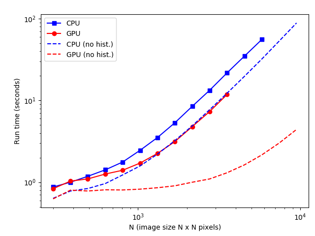
The figure shows the total run time of the script (in seconds) as a function of the image size that ranges from 300×300 pixels up to 9500×9500 pixels. These are shown for both a CPU (with 6 cores) and a GPU. For very small images the constant overheads dominate and the run times are equal. For larger images, the GPU becomes faster – but the difference is not very significant. This is mainly because the serial Python code stands for almost half of the total run time. That is related to the large amount of data contained in the angle histograms, which are also all saved to a FITS file.

We made also a lighter version of the RHT program that returns only R (for each pixel but not as a function of the position angle) and the average position angle that the kernel has calculated based on the full histograms. In this case the angle histograms are not kept in memory and are not saved to the disk. In this case (dashed curves, “no hist.”, in the figure), Python overhead is significantly reduced and the GPU runs are now more than ten times faster than the CPU runs. The largest 9500×9500 pixel image is processed on the GPU in under four seconds and most of that time is now spent on calculations within the kernels. This also suggests that, if possible, any analysis involving the full position angle histograms should be done inside the kernels, instead of writing it to external files.

The tests were run on a laptop with a six core i7-8700K CPU running at 3.70 GHz and with an Nvidia GTX-1080 GPU. Code for RHT computations with OpenCL can be found at GitHub , in the TM directory.

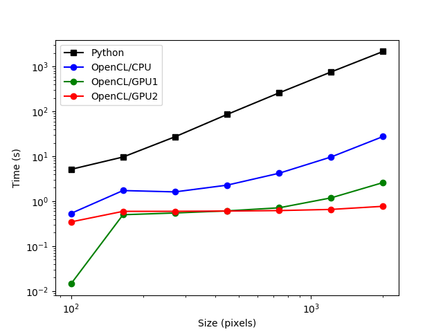
Below is are more complete comparison of the run times of the python version and the OpenCL versions. The size of the smoothing kernel and the size of the circular window are kept constant (11 and 55 pixels, respectively) and only the size of the analysed image is varied from 100×100 pixels up to 2000×2000 pixels, as indicated on the x axis. The comparison is not entirely fair because the python version also returns the angle histograms while the OpenCL routine only returns statistics derived from the histograms. However, the storage of the full histograms should not be a large factor in the overall run time (these are already computed and just not stored). The RHT calculation is particularly well suited for GPUs. The integrated GPU1 is already a factor of ten faster than the multi-core CPU. For the faster GPU2, the run time is determined by constant overheads, with no significant dependence on the image size, not yet even for images 2000×2000 pixels in size.

The tests were run on a laptop with a four core i7-8550U CPU running at 1.80GHz, an integrated Intel Corporation UHD Graphics 620 (GPU1) and an external NVidia GTX 1080 Ti (GPU2). The script test_RHT_timings.py that was used to make the above plot can be found at GitHub , in the TM subdirectory.